In nuclear medicine, a tracer molecule is administered to the patient, usually by intravenous injection. A tracer is a particular molecule, carrying an unstable isotope, a radionuclide. The molecule is recognized by the body, and will get involved in some metabolic process. The unstable isotopes produce gamma rays, which allow us to measure the concentration of the tracer molecule in the body as a function of position and time. A tracer is always administered in very low amounts, such that the natural process being studied is not affected by the tracer.
Consequently, nuclear medicine is all about measuring function or metabolism, in contrast to many other modalities including CT, MRI and echography, which mainly perform anatomical measurements. This boundary is not strict, though: CT, MRI and ultrasound imaging allow functional measurements, while nuclear medicine instruments also provide some anatomical information. However, nuclear medicine techniques provide concentration measurements with a sensitivity that is orders of magnitude higher than that of any other modality.
Radioactive decay modes
The radionuclides emit electromagnetic rays during radioactive decay. These rays are called “gamma rays” or “X-rays”. Usually, electromagnetic rays originating from nuclei are called gamma rays, while those from atoms are called x-rays. However, when they have the same frequency they are indistinguishable. The energy of a photon equals
where is the Planck constant, is the speed of light, ν the frequency and λ the wavelength of the photon. The ratio between electronvolt and joule is numerically equal to the unit of charge in coulomb: C. Visible light has a wavelength of about 400 to 700 nm, and therefore an energy of about 4.1 to 1.8 eV. The gamma rays used in nuclear medicine have energies of 100 to 600 keV, corresponding to wavelengths of a few pm.
There are many ways in which unstable isotopes can decay. Depending on the decay mode, one or more gamma rays will be emitted in every event. Some isotopes may use different decay modes. The probability of each mode is called the branching ratio. As an example, 18F has a branching ratio of 0.97 for positron decay, and a branching ratio of 0.03 for electron capture.
emission.
In this process, a neutron is transformed into a proton and an electron (called a particle). Also a neutrino (an electron anti-neutrino ) is produced and (since the decay result is more stable) some energy is released:
Since the number of protons is increased, this transmutation process corresponds to a rightward step in Mendeleev’s table.
The resulting daughter product of the above transmutation can also be in an excited state, in which case it rapidly decays to a more stable nuclear arrangement, releasing the excess energy as one or more γ photons. The nucleons are unchanged, so there is no additional transmutation in decay from excited to ground state.
The daughter nucleus of the decay process may also be in a metastable or isomeric state. In contrast to an excited state, the life time of a metastable state is “much longer” [1]
When it finally decays, it does so by emitting a photon. In many metastable isotopes, this photon may be immediately absorbed by an electron of the very same atom, as a result of which that electron is ejected. This is called a (internal) conversion electron. The kinetic energy of the ejected electron is equal to the difference between the energy of the photon and the electron binding energy.
The most important single photon isotope 99mTc is an example of this mode. 99mTc is a metastable daughter product of 99Mo (half life 66 hours). 99mTc decays to 99Tc (half life 6 hours) by emitting a photon of 140 keV. 99Mo is produced in a fission reactor [2]
Electron capture (EC).
An orbital electron is captured, and combined with a proton to produce a neutron and an electron neutrino:
As a result of this, there is an orbital electron vacancy. An electron from a higher orbit will fill this vacancy, emitting the excess energy as a photon. Note that EC causes transmutation towards the leftmost neighbor in Mendeleev’s table.
If the daughter product is in an excited state, it will further decay towards a state with lower energy by emitting additional energy as γ photons (or conversion electrons).
Similarly, the daughter product may be metastable, decaying via isomeric transition after a longer time.
Examples of radionuclides decaying with EC are 57Co, 111In, 123I and 201Tl. Figure 1 shows the decay scheme for 111In and (a small part of) the decay table. Conversion electrons are denoted with “ce-, ”, where is the electron shell and is the gamma ray. The table also gives the kinetic energy of the conversion electron, which must of course be less than the energy of the photon that produced it. The ejection of the conversion electron creates a vacancy in the involved electron shell, which is filled by an electron from a higher shell. The excess energy is released as an X-ray or as an Auger electron. In the decay table, X-rays are denoted with “ X-ray”, where is the electron shell that had a vacancy, and says (in code) from which shell the new electron comes. The energy of this X-ray exactly equals the difference between the energies of the two electron shells. Instead of emitting an X-ray, the excess energy can be used to emit another electron from the atom. This is called the Auger-effect, and the emitted electron is called an Auger-electron. In the table an Auger electron is denoted as “Auger-”, if a vacancy in shell is filled by an electron from shell , using the excess energy to emit an electron from shell . The table gives the kinetic energy of the emitted Auger-electron. The table also gives the frequency, i.e. the probability that each particular emission occurs when the isotope decays.
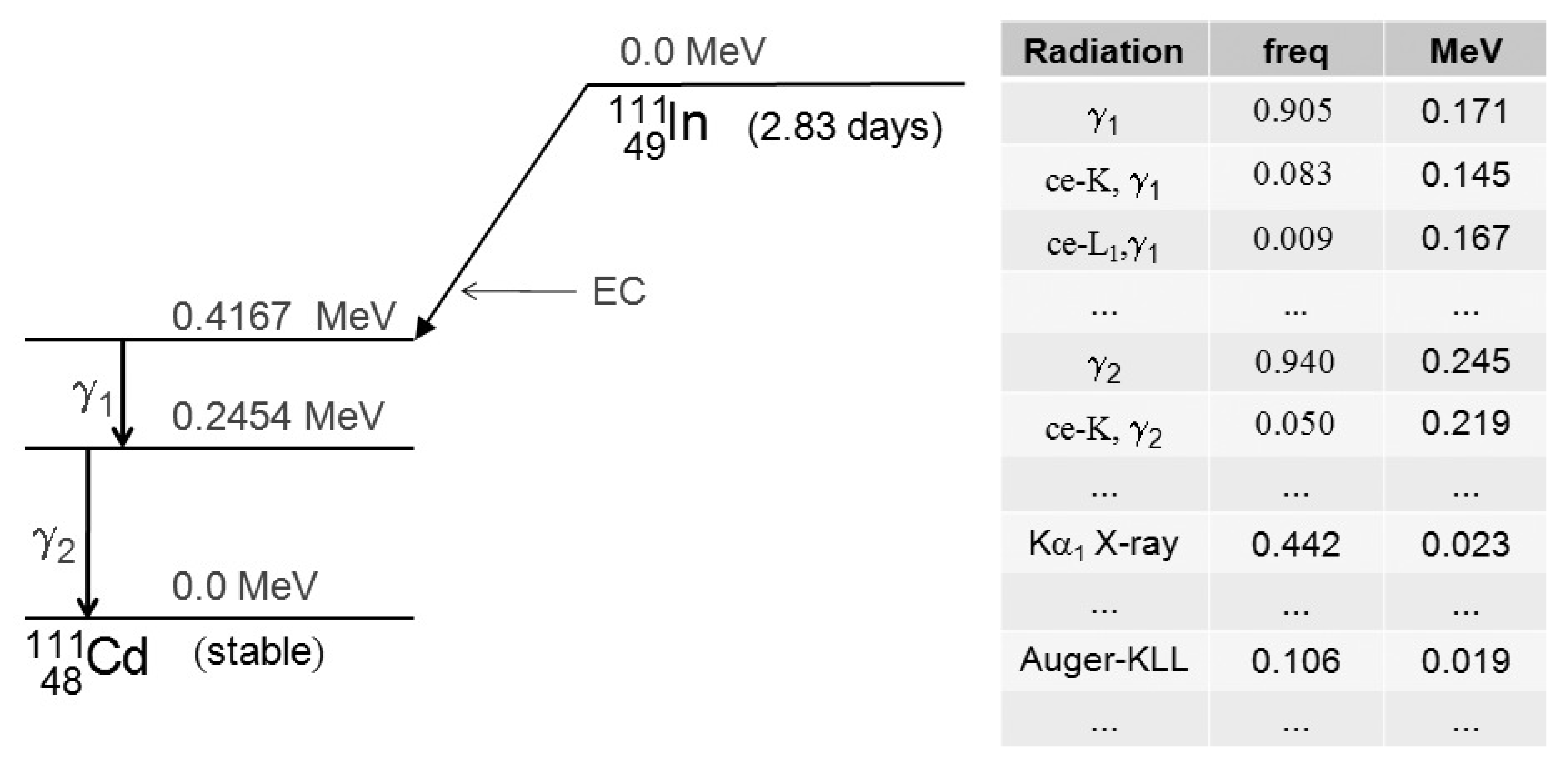
Figure 1:Decay scheme of 111In, by electron capture. The scheme is dominated by the emission of two gamma rays (171 and 245 keV). These gamma rays can be involved in production of conversion electrons. A more complete table is given in SR Cherry et al. (2012).
Positron emission ( decay).
A proton is transformed into a neutron and a positron (or anti-electron):
After a very short time the positron will hit an electron and annihilate (Figure 2). The mass of the two particles is converted into energy, which is emitted as two photons. These photons are emitted in opposite directions. Each photon has an energy of 511 keV (the rest mass of an electron or positron).
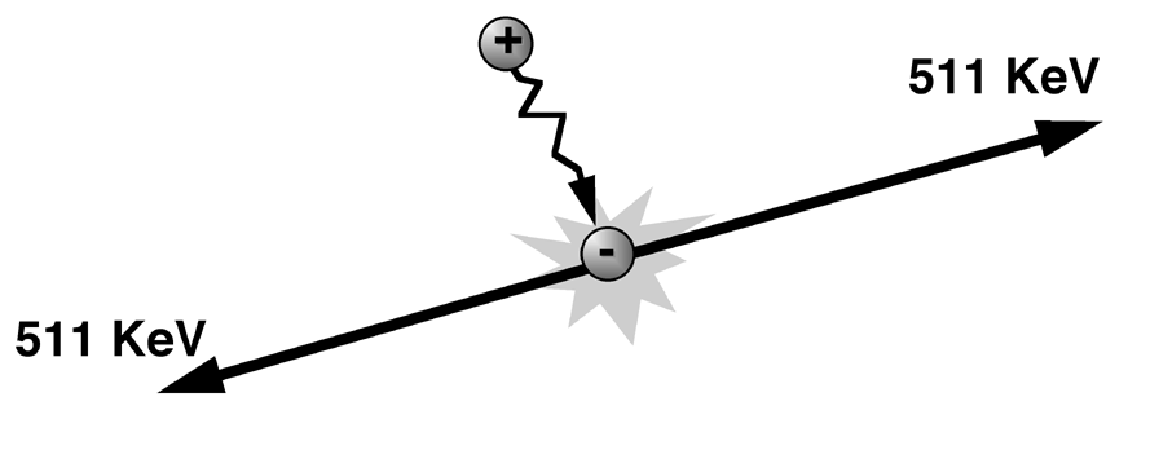
Figure 2:Positron-electron annihilation.
Again, the daughter nucleus may also be in an excited or a metastable state.


As a rule of thumb, light atoms tend to emit positrons, heavy ones tend to prefer other modes, but there are exceptions. The most important isotopes used for positron emission imaging are 11C, 13N, 15O and 18F. Since these atoms are very frequent in biological molecules, it is possible to make a radioactive tracer which is chemically identical to the target molecule, by substitution of a stable atom by the corresponding radioactive isotope. These isotopes are relatively short lived: 11C: 20 min, 13N: 10 min, 15O: 2 min and 18F: 2 hours. As a result, except for 18F, they must be produced close to the PET-system immediately before injection. To produce the isotope, a small cyclotron is required. The isotope must be rapidly incorporated into the tracer molecule in a dedicated radiopharmacy laboratory. In contrast, 18F can be transported from the production site to the hospital. That makes it the most popular isotope in PET.
In nuclear medicine, we use radioactive isotopes that emit photons with an energy between 80 and 300 keV for single photon emission, and 511 keV for positron emission. The energy of the emitted photons is fixed: each isotope emits photons with one or a few very sharp energy peaks. If more than one peak is present, each one has its own probability which is a constant for that isotope. So if we administer a tracer to a patient, we know exactly what photons we will have to measure.
Statistics
The exact moment at which an atom will decay cannot be predicted. All that is known is the probability that it will decay in the next time interval . This probability is , where α is a constant for each isotope. So if we have radioactive atoms at time , we expect to see a decrease in the next interval of
Integration over time yields
This is what we expect. If we actually measure it, we may obtain a different value, since the process is statistical. As shown below, the estimate will be better for larger .
The amount of radioactivity is not expressed as the number of radioactive atoms present, but as the number of radioactive atoms decaying per unit of time. From (5) we find that
Therefore, for the same amount of radioactivity, more radioactive atoms are needed if the half life is longer. This quantity used to be expressed in Curie (Ci), but the preferred unit is now Becquerel (Bq). Marie and Pierre Curie and Antoine Becquerel received the Nobel prize in 1903, for their discovery of radioactivity in 1896. One Bq means 1 decay per s. For the coming years, it is useful to know that
The amounts of radioactivity used in nuclear medicine imaging are typically in the order of MBq.
The half life of a tracer is the amount of time after which only half the amount of radioactivity is left. It is easy to compute it from equation (6):
As shown in appendix Poisson noise, the probability that decays occur, when decays are expected equals
This is a Poisson distribution with the average number of expected photons. The mean of the distribution is , and the standard deviation equals . For large , it can be well approximated by a Gaussian with mean and standard deviation :
For smaller ones (less than 10 or so) it becomes markedly asymmetrical, since the probability is always 0 for negative values.
Note that the distribution is only defined for integer values of . Note, however, that is a real number (the expected number of decays does not need to be an integer number). Summing over all values yields
As with a Gaussian, is not only the mean of the distribution, it is also the value with highest probability.
When one estimates radioactivity by counting emitted particles after decay, the signal-to-noise ratio (SNR = mean / standard deviation) of that measurement equals
where is the expection of the number of measured photons. Hence, if we measure the amount of radioactivity with particle detectors, the SNR becomes larger if we detect more particles (measure longer). In other words, the relative uncertainty (1/SNR = standard deviation / mean), becomes smaller if we detect more particles.
The only assumption made in the derivation in appendix Poisson noise was that the probability of an event was constant in time. It follows that “thinning” a Poisson process results in a new Poisson process. With thinning, we mean that we randomly accept or reject events, using a fixed acceptance probability. If we expect photons, and we randomly accept with a probability , then the expected number of accepted photons is . Since the probability of surviving the whole procedure (original process followed by selection) has a fixed probability, the resulting process is still Poisson.
The boundary between excited and metastable is usually said to be about s, which is rather short in practice. But the half life of some isomers is in the order of days or years.
There are only 5 places worldwide where 99Mo is produced (one in Mol, Belgium, one in Petten, the Netherlands), and 4 where it can be processed to produce 99mTc generators (one in Petten, one in Fleurus, Belgium)..
- SR Cherry, JA Sorenson, & ME Phelps. (2012). Physics in Nuclear Medicine. Saunders. 10.1016/B978-1-4160-5198-5.00001-0