Introduction
The tomographic systems are shown (once again) in Figure 1. They have in common that they perform an indirect measurement of what we want to know: we want to obtain information about the distribution in every point, but we acquire information integrated over projection lines. So the desired information must be computed from the measured data. In order to do that, we need a mathematical function that describes (simulates) what happens during the acquisition: this function is an operator that computes measurements from distributions. If we have that function, we must derive its inverse: this will be an operator that computes distributions from measurements.
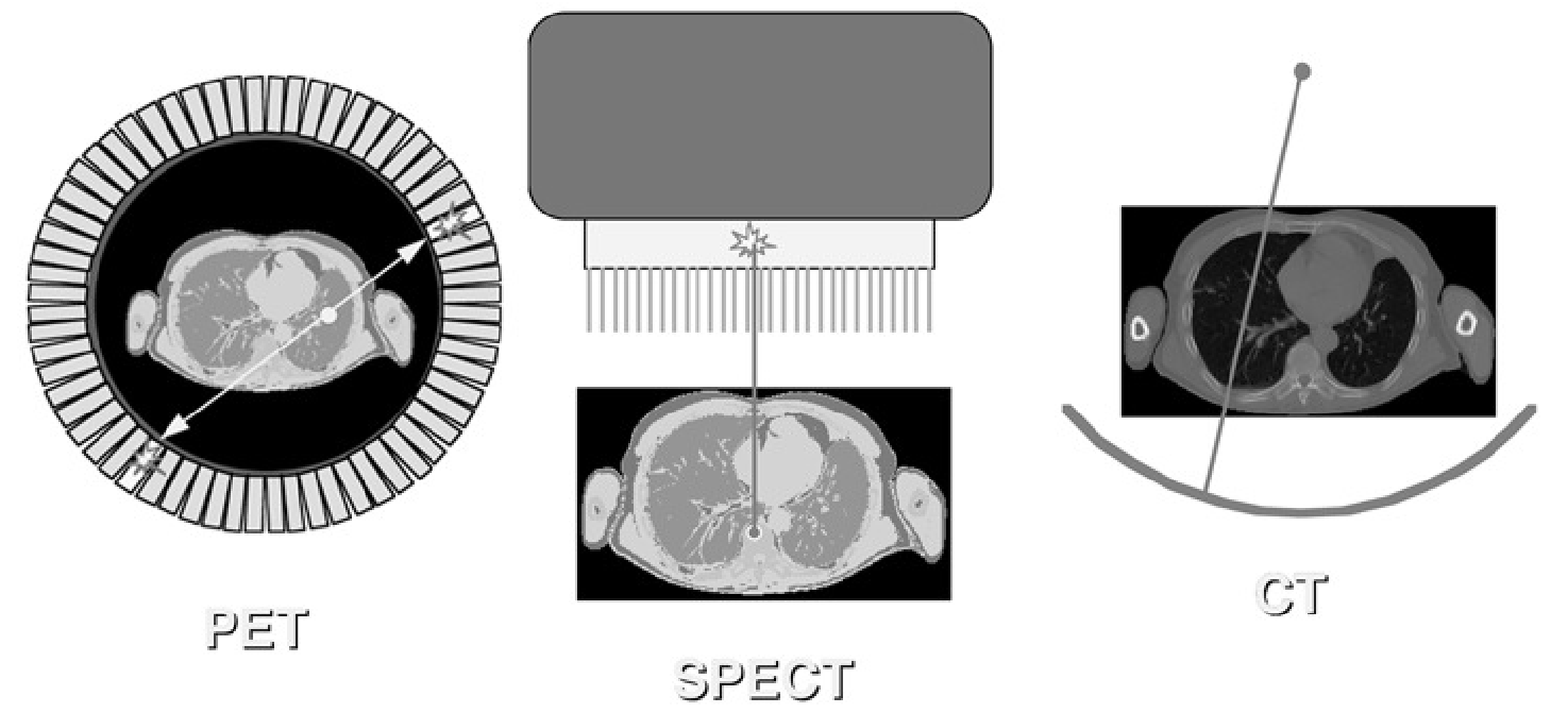
Figure 1:Information acquired along lines in the PET camera, the gamma camera and the CT-scanner.
In the previous chapters we have studied the physics of the acquisition, so we are ready to compose the acquisition model. We can decide to introduce some approximation to obtain a simple acquisition model, hoping that deriving the inverse will not be too difficult. The disadvantage is that the inverse operator will not be an accurate inverse of the true acquisition process, so the computed distribution will not be identical to the true distribution. On the other hand, if we start from a very detailed acquisition model, inverting it may become mathematically and/or numerically intractable.
For a start, we will assume that collimation is perfect and that there is no noise and no scatter. We will only consider the presence of radioactivity and attenuating tissue.
Consider a single projection line in the CT-camera. We define the -axis such that it coincides with the line. The source is at , the detector at . A known amount of photons is emitted in towards the detector element at . Only photons arrive, the others have been eliminated by attenuation. If is the linear attenuation coefficient in the body of the patient at position , we have (see also equation (5))
The exponential gives the probability that a photon emitted in towards is not attenuated and arrives safely in .
For a gamma camera measurement, there is no transmission source. Instead, the radioactivity is distributed in the body of the patient. We must integrate the activity along the -axis, and attenuate every point with its own attenuation coefficient. Assuming again that the patient is somewhere between the points and on the -axis, then the number of photons arriving in is:
where is the activity in . For the PET camera, the situation is similar, except that it must detect both photons. Both have a different probability of surviving attenuation. Since the detection is only valid if both arrive, and since their fate is independent, we must multiply the survival probabilities:
In CT, only the attenuation coefficients are unknown. In emission tomography, both the attenuation and the source distribution are unknown. In PET, the attenuation is the same for the entire projection line, while in single photon emission, it is different for every point on the line.
It can be shown (and we will do so below) that it is possible to reconstruct the planar distribution, if all line integrals (or projections) through a planar distribution are available. As you see from Figure 1, the gamma camera and the CT camera have to be rotated if all possible projections must be acquired. In contrast, a PET ring detector acquires all projections simultaneously (with “all” we mean here a sufficiently dense sampling).
Planar imaging
Before discussing how the activity and/or attenuation distributions can be reconstructed, it is interesting to have a look at the raw data. For a gamma camera equipped with parallel hole collimator, the raw data are naturally organized as interpretable images, “side views” of the tracer concentration in the transparent body of the patient. For a PET camera, the raw data can be organized in sets of parallel projections as well, as shown in Figure 2.
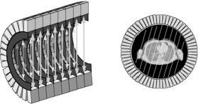
Figure 2:Raw PET data can be organized in parallel projections, similar as in the gamma camera.
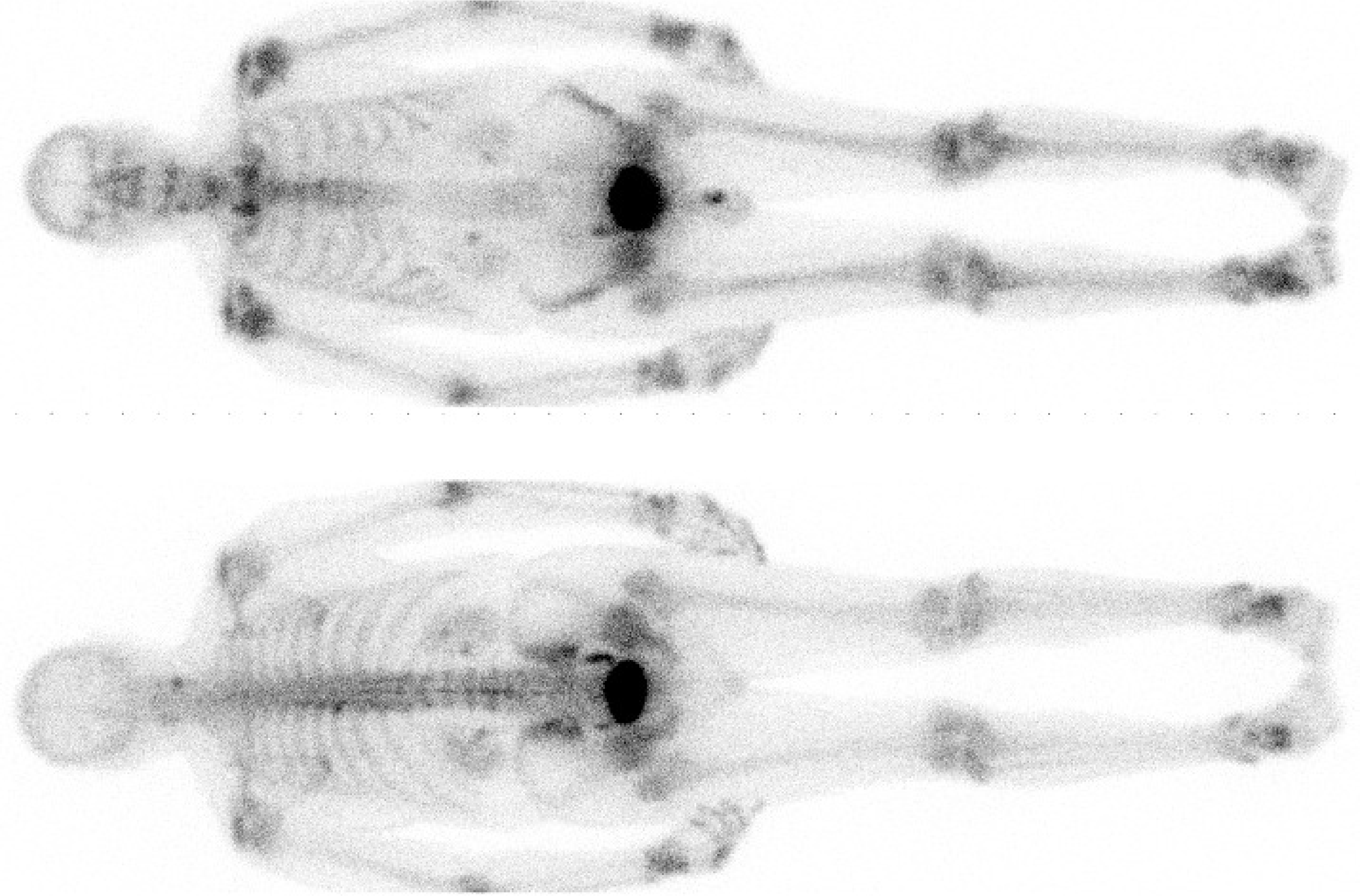
Figure 3:99mTc-MDP study acquired on a dual head gamma camera. Detector size is about 40 × 50 cm, the whole body images are acquired with slow translation of the patient bed. MDP accumulates in bone, allowing visualization of increased bone metabolism. Due to attenuation, the spine is better visualized on the posterior image.
Figure 3 shows a planar whole body image, which is obtained by slowly moving the gamma camera over the patient and combining the projections into a single image. In this case, a gamma camera with two opposed detector heads was used, so the posterior and anterior views are acquired simultaneously. There is no rotation, these are simply raw data, but they provide valuable diagnostic information. A similar approach is applied in radiological studies: with the CT tomographic images can be produced, but the planar images (e.g. thorax X-ray) already provide useful information.

Figure 4:A few images from a renography. The numbers are the minutes after injection of the 99mTc-labeled tracer. The left kidney (at the right in the image) is functioning normally, the other one is not: both uptake and clearance of the tracer are slowed down.
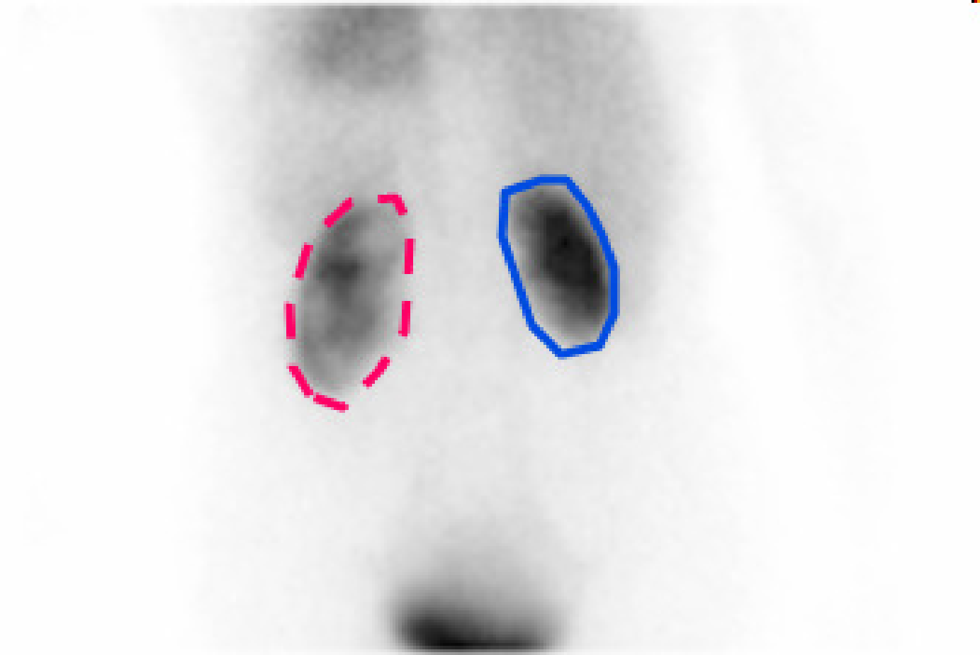
Figure 5:Summing all frames of the dynamic renal study yields the image on the left, where the kidneys can be easily delineated. The total count in these regions as a function of time (time activity curves or TACs) are shown on the right, revealing a distinct difference in kidney function.
The dynamic behaviour of the tracer can be measured by acquiring a series of consecutive images. To study the function of the kidneys, a 99mTc labeled tracer (in this example ethylene dicysteine, known as 99mTc-EC) is injected, and its renal uptake is studied over time. The first two minutes after injection, 120 images of 1 s are acquired to study the perfusion. Then, about a hundred planar images are acquired over 40 min to study the clearance. Figure 4 and Figure 5 show the results in a patient with one healthy and one poorly functioning kidney.
The study duration should not be too long because of patient comfort. A scanning time of 15 min or half an hour is reasonable, more is only acceptable if unavoidable. If that time is used to acquire a single or a few planar images, there will be many photons per pixel resulting in good signal to noise ratio, but there is no depth information. If the same time is used to acquire many projections for tomographic reconstruction, then there will be few counts per pixel and more noise, but we can reconstruct a three-dimensional image of the tracer concentration. The choice depends on the application.
In contrast, planar PET studies are very uncommon, because most PET-cameras are acquiring all projections simultaneously, so the three-dimensional image can always be reconstructed.
2D Emission Tomography
In this section, we will study the reconstruction of a planar distribution from its line integrals. The data are two-dimensional: a projection line is completely specified by its angle and its distance to the center of the field of view. A two-dimensional image that uses as the column coordinate and θ as the row coordinate is called a sinogram. Figure 6 shows that the name is well chosen: the sinogram of point source is zero everywhere except on a sinusoidal curve. The sinogram in the figure is for 180º. A sinogram for 360º shows a full period of the sinusoidal curve. It is easy to show that, using the conventions of Figure 6, , so the non-zero projections in the sinogram are indeed following a sinusoidal curve.
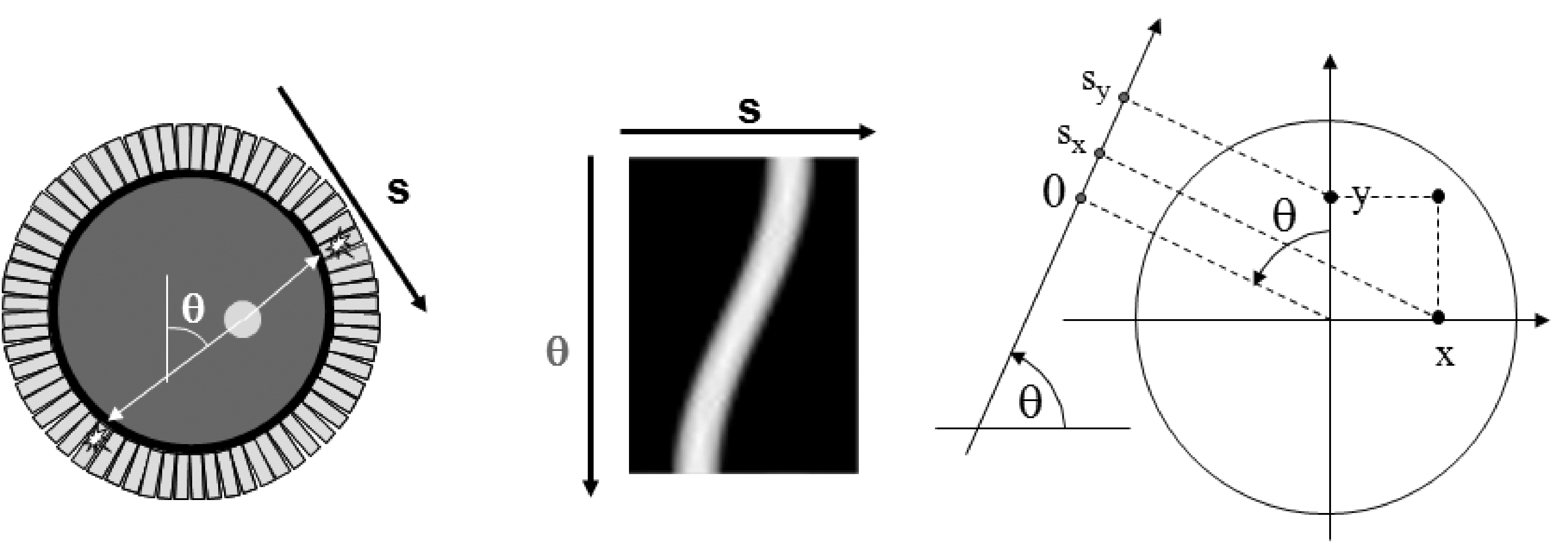
Figure 6:A sinogram is obtained by storing the 1D parallel projections as the rows in a matrix (or image). Left: the camera with a radioactive disk. Center: the corresponding sinogram. Right: the conventions, θ is positive in clockwise direction.
2D filtered backprojection
Filtered backprojection (FBP) is the mathematical inverse of an idealized acquisition model: it computes a two-dimensional continuous distribution from ideal projections. In this case, “ideal” means the following:
The distribution has a finite support: it is zero, except within a finite region. We assume this region is circular (we can always do that, since the distribution must not be non-zero within the support). We assume that this region coincides with the field of view of the camera. We select the center of the field of view as the origin of a two-dimensional coordinate system.
Projections are continuous: the projection is known for every angle and for every distance from the origin. Projections are ideal: they are unweighted line integrals (so there is no attenuation and no scatter, the PSF is a Dirac impulse and there is no noise).
The distribution is finite everywhere. That should not be a problem in real life.
Projection
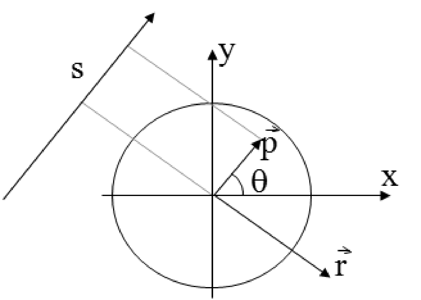
Figure 7:The projection line as a function of a single parameter . The line consists of the points , with , .
Such an ideal projection is then defined as follows (using the conventions of Figure 6):
The point is the point on the projection line closest to the center of the field of view. By adding we take a step along the projection line (Figure 7).
The Fourier theorem
The Fourier theorem (also called the central slice theorem) states that there is a simple relation between the one-dimensional Fourier transform of the projection and the two-dimensional Fourier transform of the distribution .
The Fourier theorem is very easy to prove for projection along the y-axis (so ). Because the y-axis may be chosen arbitrarily, it holds for any other projection angle (but the notation gets more elaborate). In the following is the 1-D Fourier transform (in the first coordinate) of . Because the angle is fixed and zero, we have .
Here, . Let us now compute the 2-D Fourier transform Λ of λ:
So it immediately follows that . Formulated for any angle θ this becomes:
A more rigorous proof for any angle θ is given in appendix Central slice theorem. In words: the 1-D Fourier transform of the projection acquired for angle θ is identical to a central profile along the same angle through the 2-D Fourier transform of the original distribution (Figure 8).
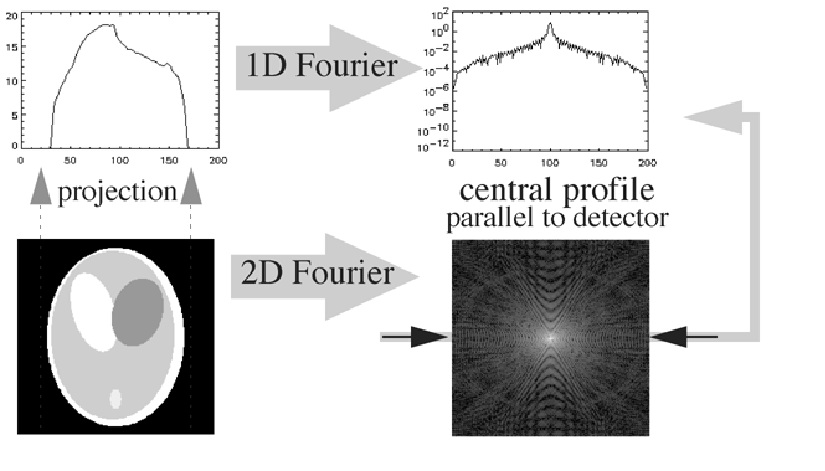
Figure 8:The Fourier theorem.
The Fourier theorem directly leads to a reconstruction algorithm by simply digitizing everything: compute the 1D FFT transform of the projections for every angle, fill the 2D FFT image by interpolation between the radial 1D FFT profiles, and compute the inverse 2D FFT to obtain the original distribution.
Obviously, this will only work if we have enough data. Every projection produces a central line through the origin of the 2D frequency space. We need to have an estimate of the entire frequency space, so we need central lines over at least 180 degrees (more is fine but redundant). Figure 9 shows clinical raw emission data acquired for tomography. They can be organized either as projections or as sinograms. There are typically in the order of 100 (SPECT) or a few hundreds (PET) of projection angles. The figure shows 9 of them. During a clinical study, the gamma camera automatically rotates around the patient to acquire projections over 180º or 360º. Because the spatial resolution deteriorates rapidly with distance to the collimator, the gamma camera not only rotates, it also moves radially as close as possible to the patient to optimize the resolution.
As mentioned before, the PET camera consisting of detector rings measures all projection lines simultaneously, no rotation is required.
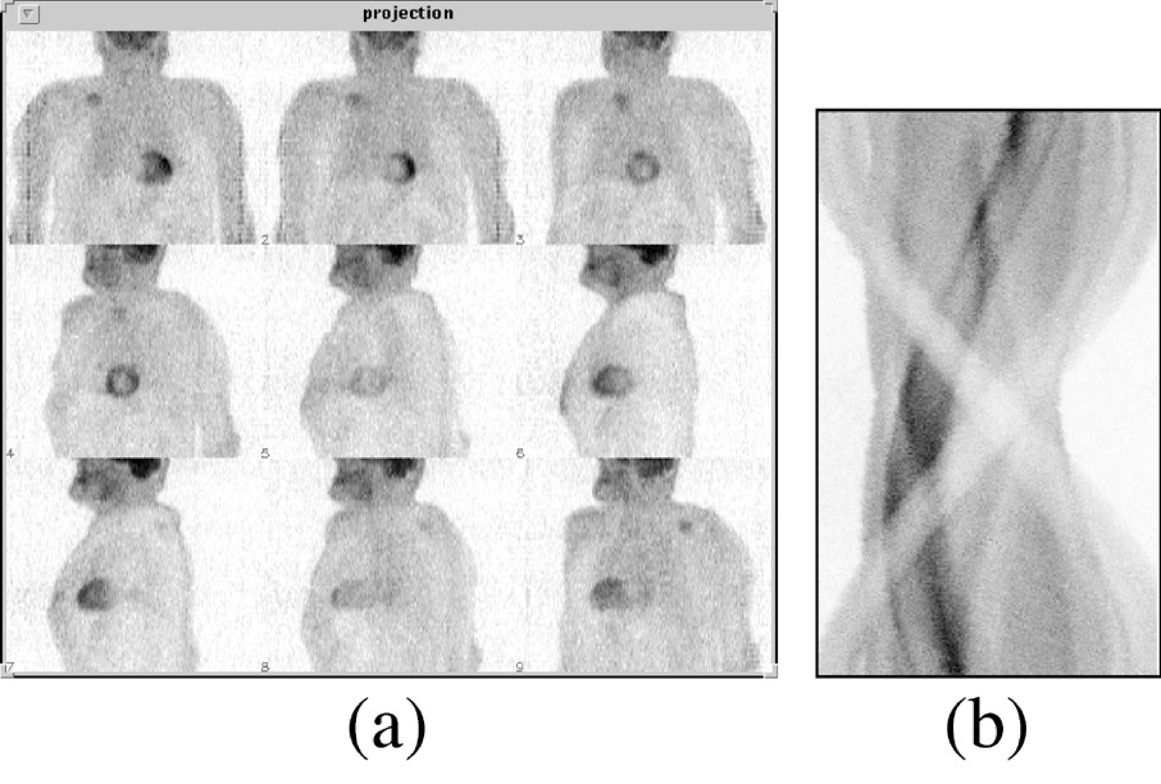
Figure 9:Raw PET data, organized as projections (a) or as a sinogram (b). There are typically a few hundred projections, one for each projection angle, and several tens to hundred sinograms, one for each slice through the patient body
Backprojection
This Fourier-based reconstruction works, but usually an alternative expression is used, called “filtered backprojection”. To explain it, we must first define the operation backprojection:
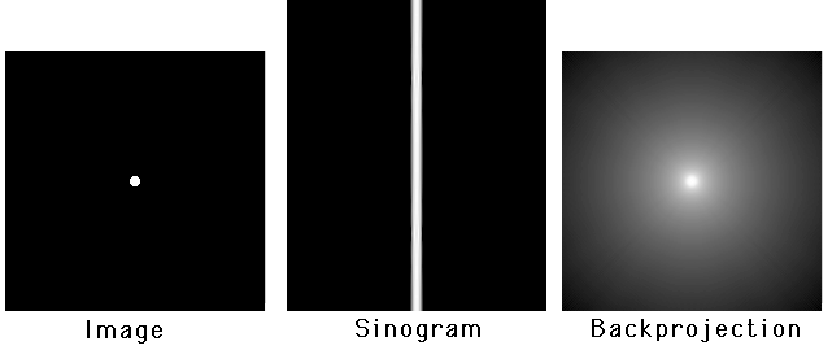
Figure 10:A point source, its sinogram and the backprojection of the sinogram (logarithmic gray value scale).
During backprojection, every projection value is uniformly distributed along its projection line. Since there is exactly one projection line passing through for every angle, the operation involves integration over all angles. This operation is NOT the inverse of the projection. As we will see later on, it is the adjoint operator of projection. Figure 10 shows the backprojection image using a logarithmic gray value scale. The backprojection image has no zero pixel values!
Let us compute the values of the backprojection image from the projections of a point source. Because the point is in the origin, the backprojection must be radially symmetrical. The sinogram is zero everywhere except for (Figure 10), where it is constant, say . So in the backprojection we only have to consider the central projection lines, the other lines contribute nothing to the backprojection image. Consider the line integral along a circle around the center (that is, the sum of all values on the circle). The circle intersects every central projection line twice, so the total activity the circle receives during backprojection is
So the line integral over a circle around the origin is a constant. The value in every point of a circle with radius is . In conclusion, starting with an image which is zero everywhere, except in the center where it equals , we find:
A more rigorous derivation is given in appendix Backprojection of a projection of a point source.
Projection followed by backprojection is a linear operation. In the idealized case considered here, it is also a shift invariant operation. Consequently, we have actually computed the point spread function of that operation.
Filtered backprojection
Filtered backprojection follows directly from the Fourier theorem:
The ramp filter is defined as the sequence of 1D Fourier transform, multiplication with the “ramp” and inverse 1D Fourier transform. To turn it into a computer program that can be applied to a real measurement, everything is digitized and 1D Fourier is replaced with 1D FFT. The ramp filter can also be implemented in the spatial domain:
where denotes convolution. This convolution filter is obtained by taking the inverse Fourier transform of the ramp filter, which is done in appendix 1 “The inverse Fourier transform of the ramp filter”. The ramp filter and the corresponding convolution mask are shown in Figure 11.
One can regard the ramp filter as a high pass filter which is designed to undo the blurring caused by backprojecting the projection, where the blurring mask is the point spread function computed in section Backprojection.
Mathematically, filtered backprojection is identical to Fourier-based reconstruction, so the same conditions hold: e.g. we need projections over 180 degrees. Note that after digitization, the algorithms are no longer identical. The algorithms have different numerical properties and will produce slightly different reconstructions. Similarly, implementing the ramp filter in the Fourier domain or as a spatial convolution will produce slightly different results after digitization.
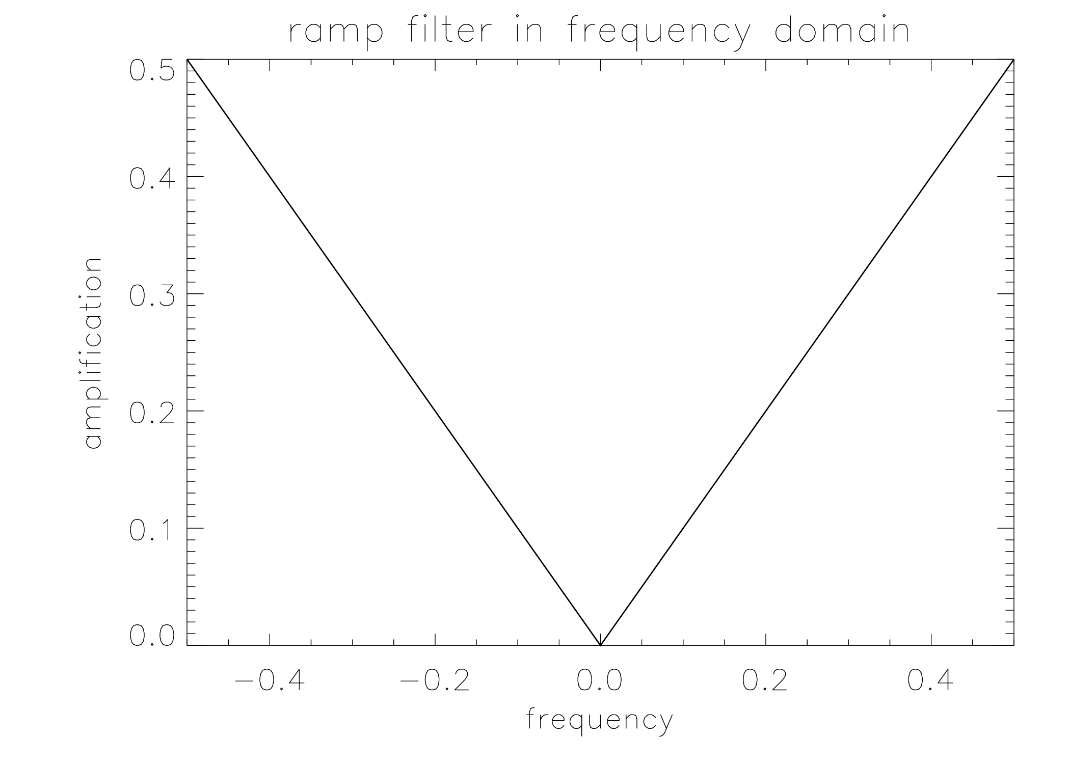
Figure 11:The rampfilter in the frequency domain (left) and its point spread function (right). The latter is by definition also the mask needed to compute the filter with a convolution in the spatial domain.
The ramp filter obviously amplifies high frequencies. If the projection data are noisy, the reconstructed image will suffer from high frequency noise. To reduce that noise, filtered backprojection is always applied in combination with a smoothing (low pass) filter.
Attenuation correction
From a CT-measurement, we can directly compute a sinogram of line integrals. Starting from (1) we obtain:
CT measurements have low noise and narrow PSF, so filtered backprojection produces good results in this case. For emission tomography, the assumptions are not valid. Probably the most important deviation from the FBP-model is the presence of attenuation.
Attenuation cannot be ignored. E.g. at 140 keV, every 5 cm of tissue eliminates about 50% of the photons. So in order to apply filtered backprojection, we should first correct for the effect of attenuation. In order to do so, we have to know the effect. This knowledge can be obtained with a measurement. Alternatively, we can in some cases obtain a reasonable estimate of that effect from the emission data only.
In order to measure attenuation, we can use an external radioactive source rotating around the patient, and use the SPECT or PET system as a CT-camera to do a transmission measurement. If the external source emits photons along the x-axis, the expected fraction of photons making it through the patient is:
This is identical to the attenuation-factor in the PET-projection, equation (4). So we can correct for attenuation by multiplying the emission measurement with the correction factor . For SPECT (equation (2)), this is not possible.
In many cases, we can assume that attenuation is approximately constant (with known attenuation coefficient μ) within the body contour. Often, we can obtain a fair body contour by segmenting a reconstruction obtained without attenuation correction. In that case, (17) can be computed from the estimated attenuation image.
Bellini has adapted filtered backprojection for constant SPECT-like attenuation within a known contour in 1979. The inversion of the general attenuated Radon transform (i.e. reconstruction for SPECT with arbitrary (but known) attenuation) has been studied extensively, but only in 2000 Novikov found a solution. The solution came a bit late in fact, because by then, iterative reconstruction had replaced analytical reconstruction as the standard approach in SPECT. And in iterative reconstruction, non-uniform attenuation poses no particular problems.
Iterative Reconstruction
Filtered backprojection is elegant and fast, but not very flexible. The actual acquisition differs considerably from the ideal projection model, and this deviation causes reconstruction artifacts. It has been mentioned that attenuation correction in SPECT may be problematic, but there are other deviations from the ideal line integral: the measured projections are not continuous but discrete, they contain a significant amount of noise (Poisson noise), the point spread function is not a Dirac impulse and Compton scatter may contribute significantly to the measurement.
That is why many researchers have been studying iterative algorithms. The nice thing about these algorithms is that they are not based on mathematical inversion. All they need is a mathematical model of the acquisition, not its inverse. Such a forward model is much easier to derive and program. That forward model allows the algorithm to evaluate any reconstruction, and to improve it based on that evaluation. If well designed, iterative application of the same algorithm should lead to continuous improvement, until the result is “good enough”.
There are many iterative algorithms, but they are rather similar, so explaining one should be sufficient. In the following, the maximum-likelihood expectation-maximization (ML-EM) algorithm is discussed, because it is currently by far the most popular one.
The algorithm is based on a Bayesian description of the problem. In addition, it assumes that both the solution and the measurement are discrete. This is correct in the sense that both the solution and the measurement are stored in a digital way. However, the true tracer distribution is continuous, so the underlying assumption is that this distribution can be well described with a discrete representation.
Bayesian approach
Assume that somehow we have computed the reconstruction Λ from the measurement . The likelihood that both the measurement and the reconstruction are the true ones () can be rewritten as:
It follows that
This expression is known as Bayes’ rule. The function is called the prior. It is the likelihood of an image, without taking into account the data. It is only based on knowledge we already have prior to the measurement. E.g. the likelihood of a patient image, clearly showing that the patient has no lungs and four livers is zero. The function is simply called the likelihood and gives the probability to obtain measurement assuming that the true distribution is Λ. The function is called the posterior. The probability is a constant value, since the data have been measured and are fixed during the reconstruction.
Maximizing is called the maximum-a-posteriori (MAP) approach. It produces “the most probable” solution. Note that this doesn’t have to be the true solution. We can only hope that this solution shares sufficient features with the true solution to be useful for our purposes.
Since it is not trivial to find good mathematical expressions for the prior probability , it is often assumed to be constant, i.e. it is assumed that a priori all possible solutions have the same probability to be correct. Maximizing then reduces to maximizing the likelihood , which is easier to calculate. This is called the maximum-likelihood (ML) approach, discussed in the following.
The likelihood function for emission tomography
We have to compute the likelihood , assuming that the reconstruction image Λ is available and represents the true distribution. In other words, how likely is it to measure with a PET or SPECT camera, when the true tracer distribution is Λ?
We start by computing what we would expect to measure. We have already done that, it is the attenuated projection from equations (2) and (4). However, we want a discrete version here:
Here, is the regional activity present in the volume represented by pixel (since we have a finite number of pixels, we can identify them with a single index). The value is the number of photons measured in detector position ( combines the digitized coordinates , it identifies a single projection line). The value represents the sensitivity of detector for activity in . If we have good collimation, is zero everywhere, except for the that are intersected by projection line , so the matrix , often called the system matrix, is very sparse. This notation is very general, and allows us e.g. to take into account the finite acceptance angle of the mechanical collimator (which will increase the fraction of non-zero ). If we know the attenuation coefficients, we can include them in the , and so on. Consequently, this approach is valid for SPECT and PET.
We now have for every detector two values: the expected value and the measured value . Since we assume that the data are samples from a Poisson distribution, we can compute the likelihood of measuring , if photons were expected (see equation (11)):
The history of one photon (emission, trajectory, possible interaction with electrons, possible detection) is independent of that of the other photons, so the overall probability is the product of the individual ones:
Obviously, this is going to be a very small number: e.g. and smaller for any other . For larger , the maximum -value is even smaller. In a measurement for a single slice, we have in the order of 10000 detector positions, so the maximum likelihood value may be in the order of , which is zero in practice. We are sure the solution will be wrong. However, we hope it will be close enough to the true solution to be useful.
Maximizing (22) is equivalent to maximizing its logarithm, since the logarithm is monotonically increasing. When maximizing over Λ, factors not depending on can be ignored, so we will drop from the equations. The resulting log-likelihood function is
It turns out that the Hessian (the matrix of second derivatives) is negative definite if the matrix has maximum rank. In practice, this means that the likelihood function has a single maximum, provided that a sufficient amount of different detector positions were used.
Maximum-Likelihood Expectation-Maximization
Since we can compute the first derivative (the gradient), many algorithms can be devised to maximize . A straightforward one is to set the first derivative to zero and solve for λ.
This produces a huge set of equations, and analytical solution is not feasible.
Iterative optimization, such as a gradient ascent algorithm, is a suitable alternative. Starting with an arbitrary image Λ, the gradient for every is computed, and a value proportional to that gradient is added. Gradient ascent is robust but can be very slow, so more sophisticated algorithms have been investigated.
A very nice and simple algorithm with guaranteed convergence is the expectation- maximization (EM) algorithm. Although the resulting algorithm is simple, the underlying theory is not. In the following we simply state that convergence is proved and only show what the EM algorithm does. The interested reader is referred to appendix The convergence of the EM algorithm for some notes on convergence.
Expected value of Poisson variables, given a single measurement
The iterative algorithm described below makes use of the expected value of a Poisson variable that contributes to a measurement. This section shows how that value is computed. Consider the experiment of Figure 12: two vials containing a known amount of radioactivity are put in front of a detector.
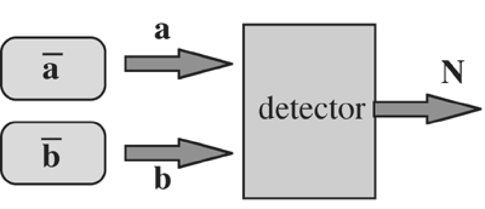
Figure 12:A detector measures the counts emitted by two sources.
Assume that we know the efficiency of the detector and its sensitivity for the two vials, so that we can compute the expected amount of photons that each of the vials will contribute during a measurement. The expected count is for vial 1 and for vial 2. Now a single experiment is carried out, and counts are measured by the detector. Question: how many photons and were emitted by each of the vials?
A-priori, we would expect photons from vial 1 and photons from vial 2. But then the detector should have measured photons. In general, because of Poisson noise. So the measurement supplies additional information, which we must use to improve our expectations about and . The answer is computed in appendix Expectation of Poisson data contributing to a measurement. The expected value of , given is:
and similar for . So if more counts were measured than the expected , the expected value of the contributing sources is “corrected” with the same factor. Extension to more than two sources is straightforward.
The complete variables
To maximize the likelihood (24), a trick is applied which at first seems to make the problem more complicated. We introduce a so-called set of “complete” variables , where is the (unknown) number of photons that have been emitted in and detected in . The are not observable, but if we would have known them, the observed variables could be computed, since . Obviously, the expected value of , given Λ is
We can now derive a log-likelihood function for the complete variables , in exactly the same way as we did for (the obey Poisson statistics, just as ). This results in:
The EM algorithm prescribes a two stage procedure (and guarantees that applying it repeatedly leads to the maximisation of both and ). It is an iterative algorithm, which starts from a given image, called , and computes an improved image . The two stages are:
Compute the function . Given and , it is impossible to compute , since we don’t know the values of . However, we can calculate its expected value, using the current estimate . This is called the E-step.
Calculate a new estimate of Λ that maximizes the function derived in the first step. This is the M-step.
The E-step
The E-step yields the following expressions:
Equation (29) is identical to equation (28), except that the unknown values have been replaced by their expected values . We would expect that equals . However, we also know that the sum of all equals the number of measured photons . This situation is identical to the problem studied in section Expected value of Poisson variables, given a single measurement, and equation (30) is the straightforward extension of equation (26) for multiple sources.
The M-step
In the M-step, we maximize this expression with respect to , by setting the partial derivative to zero:
So we find:
Substitution of equation (30) produces the ML-EM algorithm:
Discussion
This equation has a simple intuitive explanation:
The ratio compares the measurement to its expected value, based on the current reconstruction. If the ratio is 1, the reconstruction must be correct. Otherwise, it has to be improved.
The ratio-sinogram is backprojected. The digital version of the backprojection operation is
We have seen the continuous version of the backprojection in (11). The digital version clearly shows that backprojection is the transpose (or the adjoint) of projection [1]
The operations are identical, except that backprojection sums over , while projection sums over . Note that if the projection takes attenuation into account, the backprojection does so to. The backprojection does not attempt to correct for attenuation (it is not the inverse), it simply applies the same attenuation factors as in the forward projection.
Finally, the backprojected image is normalized and multiplied with the current reconstruction image. It is clear that if the measured and computed sinograms are identical, the entire operation has no effect. If the measured projection values are higher than the computed ones, the reconstruction values tend to get increased.
If the initial image is non-negative, then the final image will be non-negative too, since all factors are non-negative. This is in most applications a desirable feature, since the amount of radioactivity cannot be negative.
Comparing with (25) shows that the ML-algorithm is really a gradient ascent method. It can be rewritten as
So the gradient is weighted by the current reconstruction value, which is guaranteed to be positive (negative radioactivity is meaningless). To make it work, we can start with any non-zero positive initial image, and iterate until the result is “good enough”. Figure 13 shows the filtered backprojection and ML-EM reconstructions from the same dataset. (The image shown is not the true maximum likelihood image, since iterations were stopped early as discussed below).
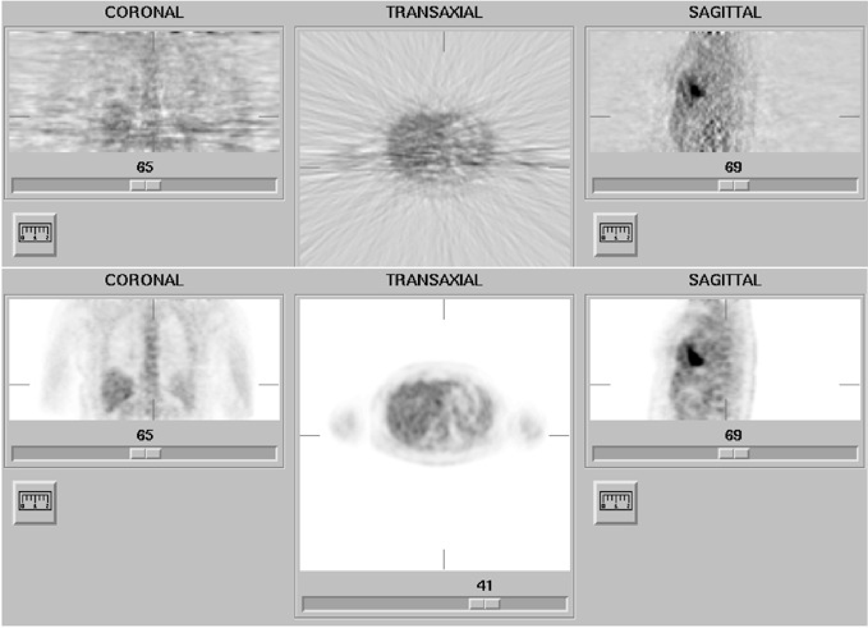
Figure 13:Reconstruction obtained with filtered backprojection (top) and maximum-likelihood expectation-maximization (34 iterations) (bottom). The streak artifacts in the filtered backprojection image are due to the statistical noise on the measured projection (Poisson noise).
Compton scatter, random coincidences
As explained in section Random coincidence correction, an estimate of the randoms contribution to the PET sinogram can be obtained, e.g. with the delayed window technique. Similarly, various methods exist to estimate the scatter contribution in SPECT (section Gamma camera) and PET (section PET camera). If an estimate of such an additive contribution to the sinogram is available, it can be incorporated in the ML-EM algorithm. The forward acquisition model of (20) is then extended as
where represents the estimate of the additive contribution from scatter and/or randoms for projection line . It can be shown that the ML-EM algorithm then becomes
Regularization
Since the levels of radioactivity must be low, the number of detected photons is also low. As a result, the uncertainty due to Poisson noise is important: the data are often very noisy.
Note that Poisson noise is “white”. This means that its (spatial) frequency spectrum is flat. Often this is hard to believe: one would guess it to be high frequency noise, because we see small points, no blobs or a shift in mean value. That is because our eyes are very good at picking up high frequencies: the blobs and the shift are there all right, we just don’t see them.
Filtered backprojection has not been designed to deal with Poisson noise. The noise propagates into the reconstruction, and in that process it is affected by the ramp filter, so the noise in the reconstruction is not white, it is truly high frequency noise. As a result, it is definitely not Poisson noise. Figure 13 clearly shows that Poisson noise leads to streak artifacts when filtered backprojection is used.
ML-EM does “know” about Poisson noise, but that does not allow it to separate the noise from the signal. In fact, MLEM attempts to compute how many of the detected photons have been emitted in each of the reconstruction pixels . That must produce a noisy image, because photon emission is a Poisson process. What we really would like to know is the tracer concentration, which is not noisy.
Because our brains are not very good at suppressing noise, we need to do it with the computer. Many techniques exist. One can apply simple smoothing, preferably in three dimensions, such that resolution is approximately isotropic. It can be shown that for every isotropic 3D smoothing filter applied after filtered backprojection, there is a 2D smoothing filter, to be applied to the measured data before filtered backprojection, which has the same effect. Since 2D filtering is faster than 3D filtering, it is common practice to smooth before filtered backprojection.
The same is not true for ML-EM: one should not smooth the measured projections, since that would destroy the Poisson nature. Instead, the images are often smoothed afterwards. Another approach is to stop the iterations before convergence. ML-EM has the remarkable feature that low frequencies converge faster than high ones, so stopping early has an effect similar to low-pass filtering.
Finally, one can go back to the basics, and in particular to the Bayesian expression (19). Instead of ignoring the prior, one can try and define some prior probability function that encourages smooth solutions. This leads to maximum-a-posteriori (MAP) algorithm. The algorithms can be very powerful, but they also have many parameters and tuning them is a delicate task.
Although regularized (smoothed) images look much nicer than the original ones, they do not contain more information. In fact, they contain less information, since low-pass filtering kills high-frequency information and adds nothing instead! Deleting high spatial frequencies results in poorer resolution (wider point spread function), so excessive smoothing is ill advised if you hope to see small structures in the image.
Convergence
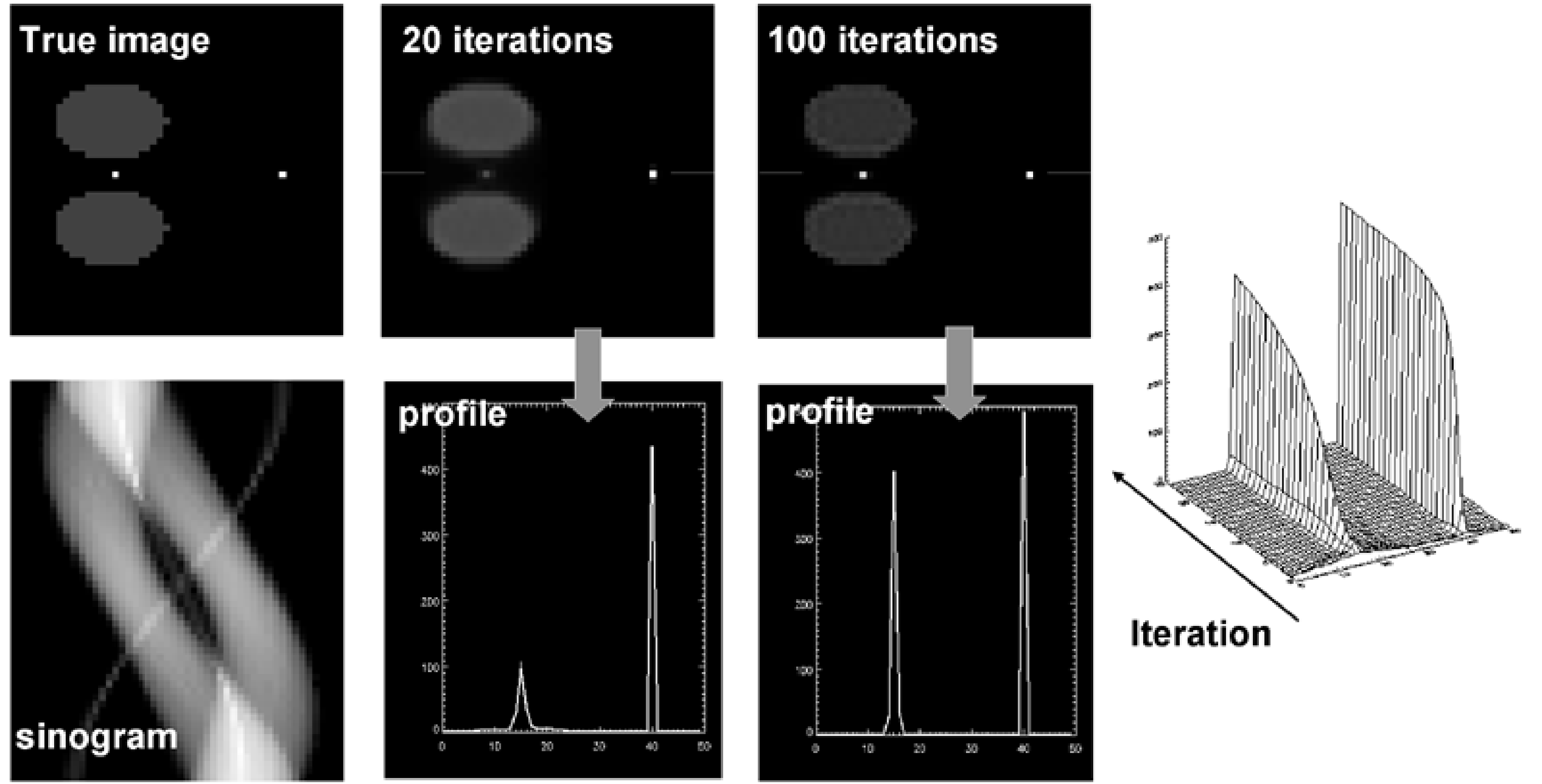
Figure 14:Simulation designed to challenge convergence of MLEM: the point between the hot regions convergence very slowly relative to the other point. The maximum converges slower than the width, so counts are not preserved.
Filtered backprojection is a linear algorithm with shift invariant point spread function. That means that the effect of projection followed by filtered backprojection can be described with a single PSF, and that the reconstruction has a predictable effect on image resolution. Similarly, smoothing is linear and shift invariant, so the combined effect of filtered backprojection with low pass filtering has a known effect on the resolution.
In contrast to FBP, MLEM algorithm is non-linear and not shift invariant. Stated otherwise, if an object is added to the reconstruction, then the effect of projection followed by reconstruction is different for all objects in the image. In addition, two identical objects can be reconstructed differently because they are at a different position. In this situation, it is impossible to define a PSF, projection followed by MLEM-reconstruction cannot be modeled as a convolution. There is no easy way to predict the effect of MLEM on image resolution.
It is possible to predict the resolution of the true maximum likelihood solution, but you need an infinite number of iterations to get there. Consequently, if iterations are stopped early, convergence may be incomplete. There is no way to tell that from the image, unless you knew a-priori what the image was: MLEM images always look nice. So stopping iterations early in patient studies has unpredictable consequences.
This is illustrated in a simulation experiment shown in Figure 14. There are two point sources, one point source is surrounded by large active objects, the other one is in a cold region. After 20 MLEM iterations, the “free” point source has nearly reached its final value, while the other one is just beginning to appear. Even after 100 iterations there is still a significant difference. The difference in convergence affects not only the maximum count, but also the total count in a region around the point source.
Consequently, it is important to apply “enough” iterations, to get “sufficiently” close to the true ML solution. In the previous section it was mentioned that stopping iterations early has a noise-suppressing effect.
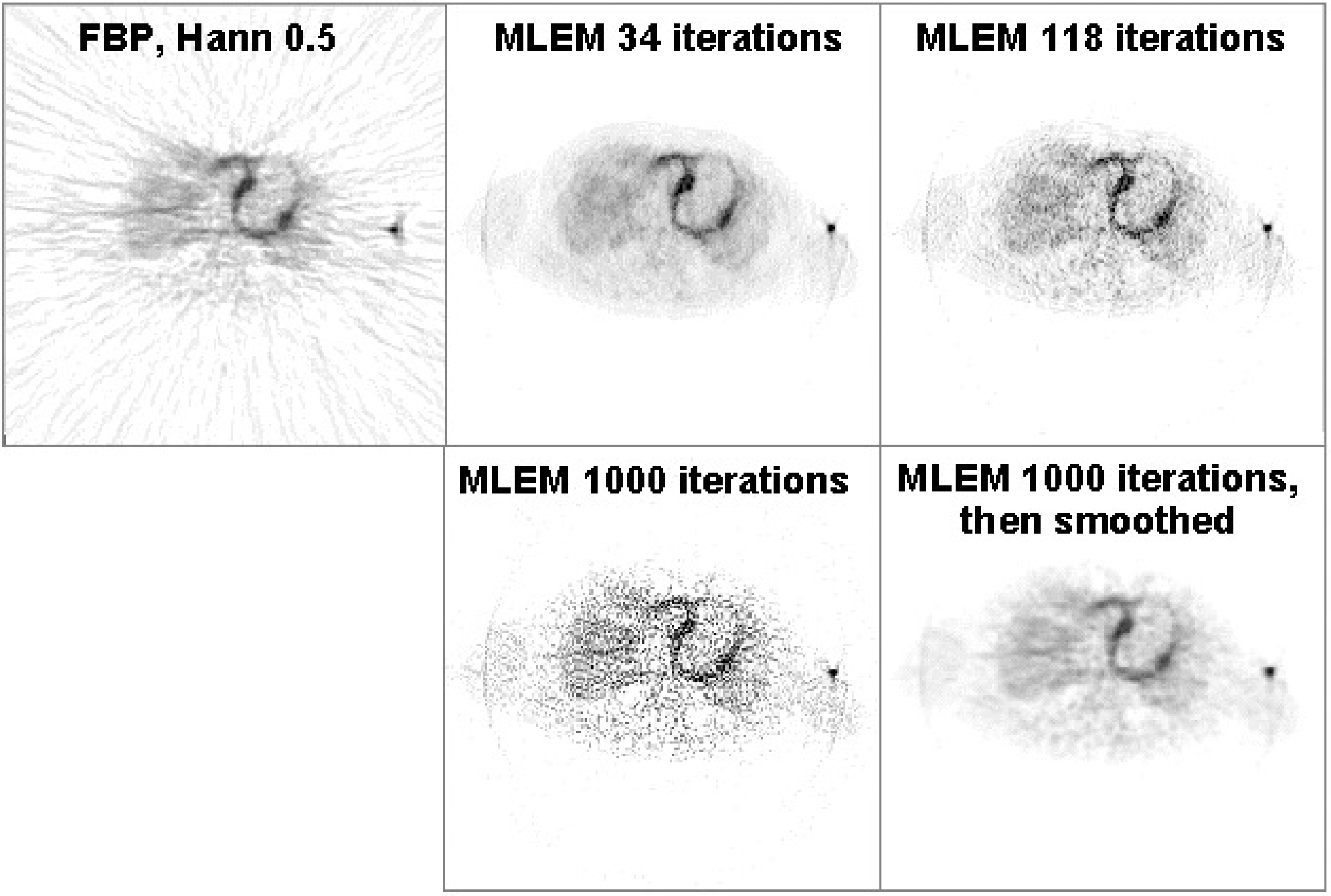
Figure 15:Reconstruction of a cardiac PET scan with FBP, and with MLEM. The images obtained after 34, 118 and 1000 iterations are shown. The image at 1000 iterations is very noisy, but a bit of smoothing turns it into a very useful image.
This is illustrated in Figure 15. After 34 MLEM iterations a “nice” image is obtained. After 1000 iterations, the image is very noisy. However, this noise is highly correlated, and drops dramatically after a bit of smoothing (here with a Gaussian convolution mask).
From Figure 14 and Figure 15 it follows that it is better to apply many iterations and remove the noise afterwards with post-smoothing. In practice, “many” is at least 30 iterations for typical SPECT and PET images, but for some applications it can mean several hundreds of iterations. One finds that when more effects are included in the reconstruction (such as attenuation, collimator blurring, scatter, randoms...), more iterations are needed. The number also depends on the image size, more iterations are needed for larger images. So if computer time is not a problem, it is recommended to apply really many iterations (several hundreds) and regularize with a prior or with post-smoothing.
OSEM

Figure 16:Illustration of OSEM: there are 160 projections in the sinogram, for an acquisition over 360º. OSEM used 40 subsets of 4 projections each, the first subset has projections at 0º, 90º, 180º and 270º. The second subset starts at 45º and so on. One OSEM iteration has 40 subiterations. The top row shows the first few and the last subiteration of OSEM. The bottom row shows the corresponding MLEM-iterations, where all projections are used for each iteration.
In each iteration, MLEM must compute a projection and a backprojection, which is very time consuming. FBP is much faster, it uses only a single backprojection, the additional cpu-time for the ramp filtering is small. Consequenly, the computation of 30 MLEM iterations takes about 60 times longer than an FBP reconstruction. MLEM was invented by Shepp and Vardi in 1982, but the required cpu time prohibited application in clinical routine. Only after 1992 clinical application started, partly because the computers had become more powerful, and partly because a very simple acceleration trick was proposed by Hudson and Larkin. The trick is called “ordered subsets expectation maximisation (OSEM)”, and the basic idea is to use only a part of the projections in every ML-iteration. This is illustrated in Figure 16. In this example, there are 160 projections, which are divided in 40 subsets of 4 projections per subset. The first subset contains the projections acquired at 0º, 90º, 180º and 270º. The second subset has the projections at 45º, 135º, 225º and 315º and so on. One OSEM iteration consists of 40 subiterations. In the first subiteration, the projection and backprojection is restricted to the first subset, the second subiteration only uses the second subset and so on. After the last subiteration, all projections have been used once. As shown in Figure 16, 1 OSEM iteration with 40 subsets produces an image very similar to that obtained with 40 MLEM iterations. Every MLEM iteration uses all projections, so in this example, OSEM obtains the same results 40 times faster.
A single OSEM iteration can be written as
where is subset . Usually, one chooses the subsets such that every projection is in exactly one subset.
The characteristics of OSEM have been carefully studied, both theoretically and in practice. In the presence of noise, it does not converge to a single solution, but to a so-called limit cycle. The reason is that the noise in every subset is different and “incompatible” with the noise in the other subsets. As a result, every subset asks for a (slightly) different solution, and in every subiteration, the subset in use “pulls” the image towards its own solution. More sophisticated algorithms with better or even guaranteed convergence have been proposed, but because of its simplicity and good performance in most cases, OSEM is now by far the most popular ML-algorithm on SPECT and PET systems.
Fully 3D Tomography
Until now, we have only discussed the reconstruction of a single 2D slice from a set of 1D projection data. An entire volume can be obtained by reconstructing neighboring slices. This is what happens in SPECT with parallel hole or fan beam collimation, in 2D PET and in single slice CT.
In some configurations this approach is not possible and the problem has to be treated as a fully three-dimensional one. There are many different geometries of mechanical collimators, and some of these acquire along lines that cannot be grouped in parallel sets. Examples are the cone beam and pinhole collimators in SPECT (Figure 5). Another example is 3D PET (section 2D and 3D PET). Three approaches to fully 3D reconstruction are discussed below.
Note that the terminology may create some confusion about the dimensions. 2D PET actually generates 3D sinogram data: the dimensions are the detector and the projection angle (defining the projection line within one slice), and the position of slice. Fully 3D PET produces 4D sinogram data. The PET detector covers typically a cylindrical surface. Two coordinates are needed to identify a single detector, hence four coordinates are needed to identify a projection line between a pair of detectors. And as will be discussed later, a series of images can be acquired over time (dynamic acquisitions), which adds another dimension to the data.
Filtered backprojection
Filtered backprojection can be extended to the fully 3D PET case. The data are backprojected along their detection lines, and then filtered to undo the blurring effect of backprojection. This is only possible if the sequence of projection and backprojection results in a shift-invariant point spread function. And that is only true if every point in the reconstruction volume is intersected by the same configuration of measured projection lines.
This is often not the case in practice. Points near the edge of the field of view are intersected by fewer measured projection lines. In this case, the data may be completed by computing the missing projections as follows. First a subset of projections that meets the requirement is selected and reconstructed to compute a first (relatively noisy) reconstruction image. Next, this reconstruction is forward projected along the missing projection lines, to compute the missing data. Then, the computed and measured data are combined into a single set of data, that now meets the requirement of shift-invariance. Finally, this completed data set is reconstructed with 3D filtered backprojection.
ML-EM reconstruction
ML-EM can be directly applied to the 3D data set: the formulation is very general, the coefficients in (33) can be directly used to describe fully 3D projection lines.
In every iteration, we have to compute a projection and a backprojection along every individual projection line. As a result, the computational burden may become pretty heavy for a fully 3D configuration.
Fourier rebinning
In PET, a rebinning algorithm is an algorithm that resamples the data in the sinogram space, so as to reorganize them into a form that leads to a simpeler reconstruction.
In 1997, an exact rebinning algorithm, called Fourier rebinning, was derived. It converts a set of 3D data into a set of 2D projections. Because all photons acquired in 3D are used to compute the rebinned 2D data set, the noise in this data set is much lower than in the corresponding 2D subset, which is a part of the original 3D data.
These projections can be reconstructed with standard 2D filtered backprojection. It was also shown that the Poisson nature of the data is more or less preserved. Consequently, the resulting 2D set can be reconstructed successfully with the 2D ML-EM algorithm as well. (Fourier rebinning is based on a wonderful feature of the Fourier transform of the sinograms, hence its name.)
In practice, the exact rebinning algorithm is not used. Instead, one only applies an approximate expression derived from it, because it is much faster and sufficiently accurate for most configurations. This algorithm (called FORE) is available on all commercial PET systems.
Time-of-flight PET
The speed of light is c = 30 cm/ns. Suppose that a point source is put exactly in the center between two PET detectors, which are connected to coincidence electronics. If two photons from the same annihilation are detected, then they must have arrived simultaneously in the respective detectors. However, the timing will be different if the source is moved 15 cm towards one detector. The photon will arrive in that detector 0.5 ns earlier, the other photon will arrive in the other detector 0.5 ns later. Consequently, if the electronics can measure the difference in arrival times , then the position of the annihilation along the projection line can be deduced: , where is the distance to the center. Using this principle in PET is called time-of-flight PET or TOF-PET.
In the eighties, TOF-PET scanners were built, but their performance was disappointing. To obtain a reasonable TOF resolution, one needs to measure the arrival time very accurately. Consequently, crystal detectors with a very short scintillation time must be used. Such crystals were available (e.g. CsF), but these fast crystals all had a poor stopping power (low attenuation coefficient) at 511 keV. Consequently, the gain obtained from the TOF-principle was more than offset by the loss due to the decreased detection sensitivity. For that reason, TOF was abandoned, and nearly all commercial PET scanners were built using BGO, which has a very high stopping power but a long scintillation time (see Table 1).
More recently, new scintillation crystals have been found, which combine high stopping power with fast scintillation decay (Table 1). In current scanners, LSO (or LYSO) is mostly used. And since the eighties, the electronics have become faster as well. The current commercial TOF-PET systems have a TOF resolution ranging from around 400 ps (6.0 cm) for older systems to around 200 ps for new systems (new in 2020).
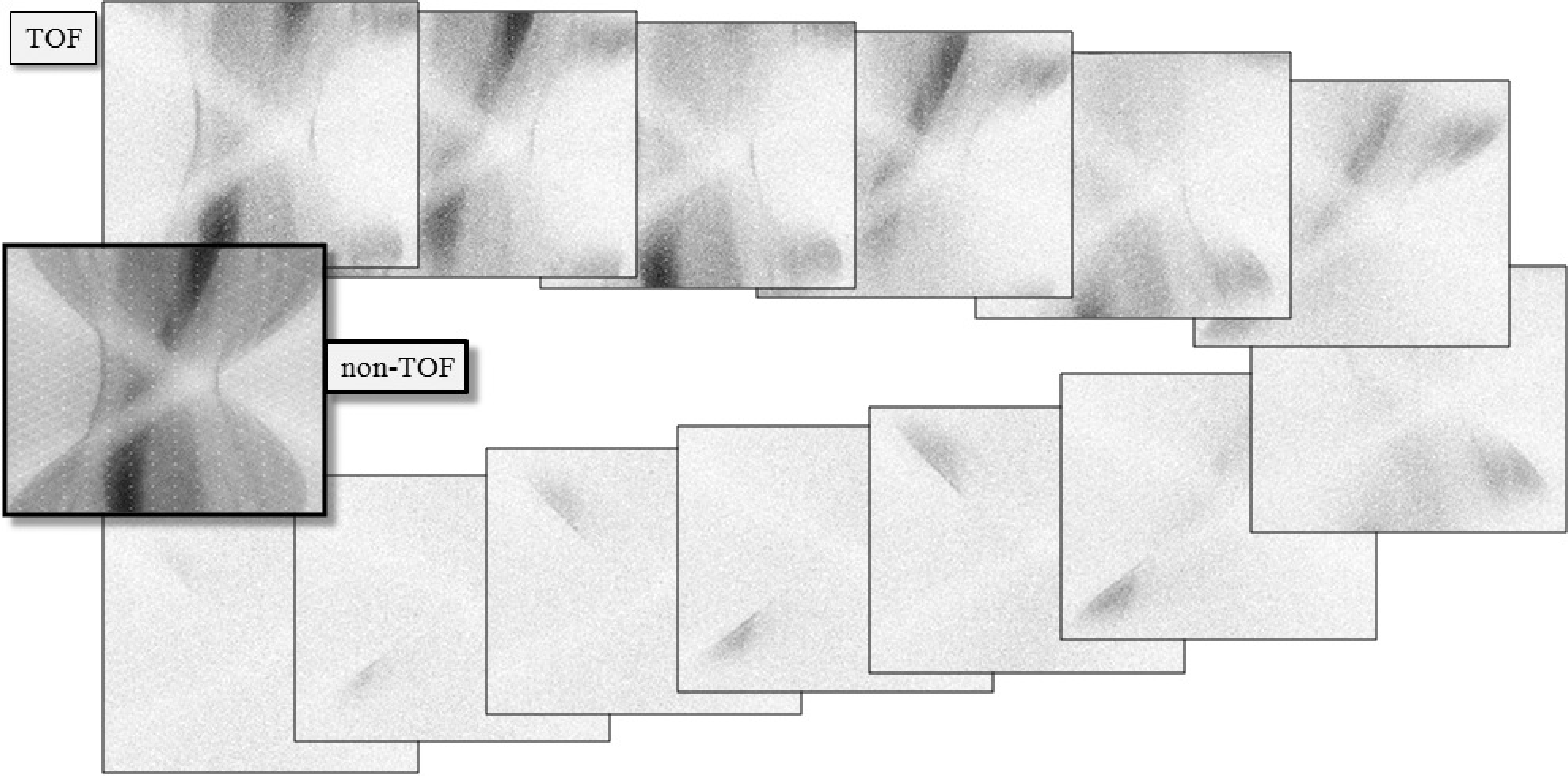
Figure 17:A single plane from a clinical TOF-data set, sampled at 13 TOF-bins. The first bin corresponds to the center, the subsequent bins are for increasing distances, alternatedly in both directions. The non-TOF sinogram was obtained by summing the 13 TOF-sinograms.
TOF-PET sinograms (or projections) have one dimension more than the corresponding non-TOF data, because with TOF, the position along the projection line is estimated as well. Figure 17 shows a TOF sinogram (sampled at 13 TOF-bins) together with the non-TOF sinogram (obtained by adding all TOF-bins).
Consequently, a parallel projection of a 2D image along a single projection angle, is not a 1D profile but a 2D image. This projection can be considered as a blurred version of the original image, where the blurring represents the uncertainty due to the point spread function of the TOF-position measurement. This can be well modeled as a 1D Gaussian blurring, as illustrated in Figure 18.
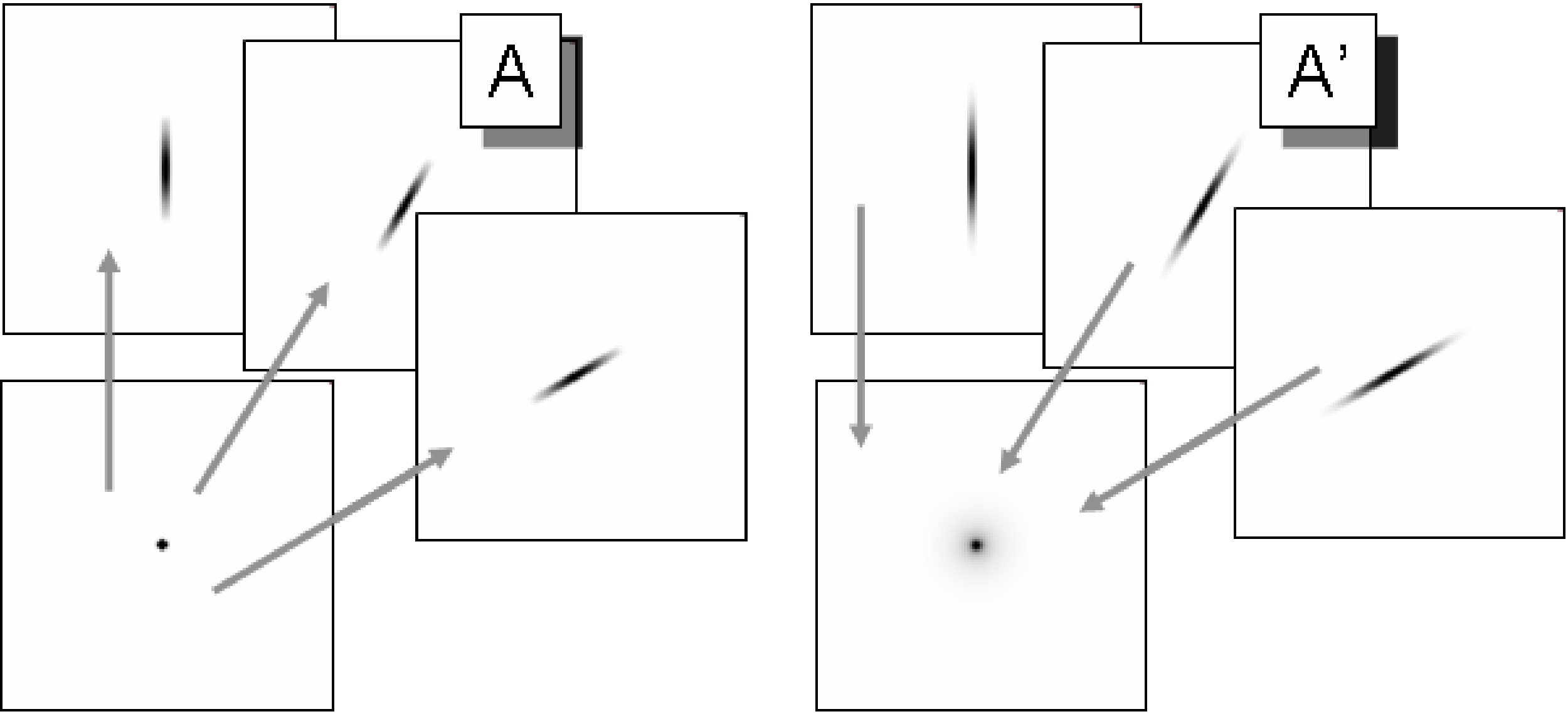
Figure 18:Left: TOF-PET projection (matrix A) can be considered as a 1D smoothing along the projection angle. Right: the TOF-PET backprojection of TOF-PET projection is equivalent to a 2D blurring filter. The blurring is much less than in the non-TOF case (Figure 10).
For iterative reconstruction, one will need the corresponding backprojection operator. Using the discrete representation, the projection can be written as:
which is the same expression as for non-TOF-PET and SPECT equation (20), but of course, the elements of the system matrix are different. The corresponding backprojection is then given by
The transpose of a symmetrical blurring operator is the same blurring operator. Consequently, every TOF-projection image must be blurred with its own 1D blurring kernel, and then they all have to be summed to produce the backprojection image. The PSF of projection followed by backprojection then yields a circularly symmetrical blob with central profile
where is the distance to the center of the blob, σ is the standard deviation of the Gaussian blurring that represents the TOF resolution, and Gauss() is a Gaussian with standard deviation , evaluated in . The standard deviation in (41) is and not simply σ, because the blurring has been applied twice, once during projection and once during backprojection. See appendix Backprojection of a projection of a point source for a more mathematical derivation.
For very large σ, this reduces to , which is the result for backprojection in non-TOF PET, obtained just after equation (12). The projection and backprojection operators are illustrated in Figure 18.
Also for TOF-PET, filtered backprojection algorithms can be developed. Because of the data redundancy, different versions of FBP can be derived. A natural choice is to use the same backprojector as mentioned above. With this backprojector, the backprojection of the TOF-PET measurement of a point source will yield the image of blob given by equation (41). Consequently, the reconstruction filter can be obtained by computing the inverse operator of (41). As before, the filter can be applied before backprojection (in the sinogram) or after backprojection (in the image), because of the Fourier theorem.

Figure 19:CT and TOF-PET image, acquired on a PET/CT system with time-of-flight resolution of about 700 ps. The TOF-PET image reveals a small lesion not seen on the non-TOF PET image. (Courtesy Joel Karp and Samuel Matej, University of Pennsylvania. The image is acquired on a Philips Gemini TOF-PET system)
Figure 19 compares a TOF and non-TOF image. By discarding the TOF-information, TOF-PET data can be converted to regular PET data. This was done here to illustrate the improvement obtained by using TOF. There are several reasons why the TOF-PET image is better.
First, because more information is used during reconstruction, the noise propagation is reduced, resulting in a better signal-to-noise ratio (less noise for the same resolution) in the TOF image. It has been shown that, for the center of a uniform cylinder, improving the TOF resolution with a factor reduces the variance in the reconstructed image with that same factor, at least if these images have the same spatial resolution.
Second, it turns out that the convergence of the MLEM algorithm is considerably faster for TOF-PET. It is known that MLEM converges faster for smaller images, because the correct reconstruction of a pixel depends on the reconstruction of all other pixels that share some projection lines with it. The TOF information reduces that number of information-sharing pixels considerably. Because in clinical routine, usually a relatively low number of iterations is applied, small image detail (high spatial frequencies) may suffer from incomplete convergence. It was found that after introducing TOF, the spatial resolution of the clinical images was better than before. TOF has no direct effect on the spatial resolution, but for a similar number of iterations, MLEM converges faster, producing a better resolution. And because of the improved SNR, it can achieve this better resolution at a similar or better noise level than non-TOF PET.
Third, an additional advantage of this reduced dependency on other pixels is a reduced sensitivity to most things that may cause artifacts, such as errors in the attenuation map, patient motion, data truncation and so on. In non-TOF PET, the resulting artifacts can propagate through the entire image. In TOF-PET, that propagation is reduced because of the reduced dependencies between the reconstructed pixel values.
Finally, the gain due to TOF is higher when the region of interest is surrounded by more activity and if the active object (i.e. the patient body) is larger. The reason is that in those cases, there is more to be gained by suppressing sensitivity to surrounding activity, since there is more surrounding activity. As a result, TOF helps more in situations where non-TOF MLEM performs poorest. The opposite is also true, for imaging a point source, TOF-PET does not better than non-TOF PET.
Reconstruction with resolution modeling
In every MLEM iteration a projection and backprojection is executed. The projection simulates the acquisition and the backprojection is the corresponding adjoint operator. A more accurate simulation of the acquisition should result in a more accurate reconstruction of the image from the acquired tomographic data. In SPECT, the system matrix elements should account for the position dependent attenuation to ensure that MLEM produces quantitative images. In PET, the elements should model the attenuation and detector sensitivities (see equation (30)), and for TOF-PET, also the width of the TOF-resolution.
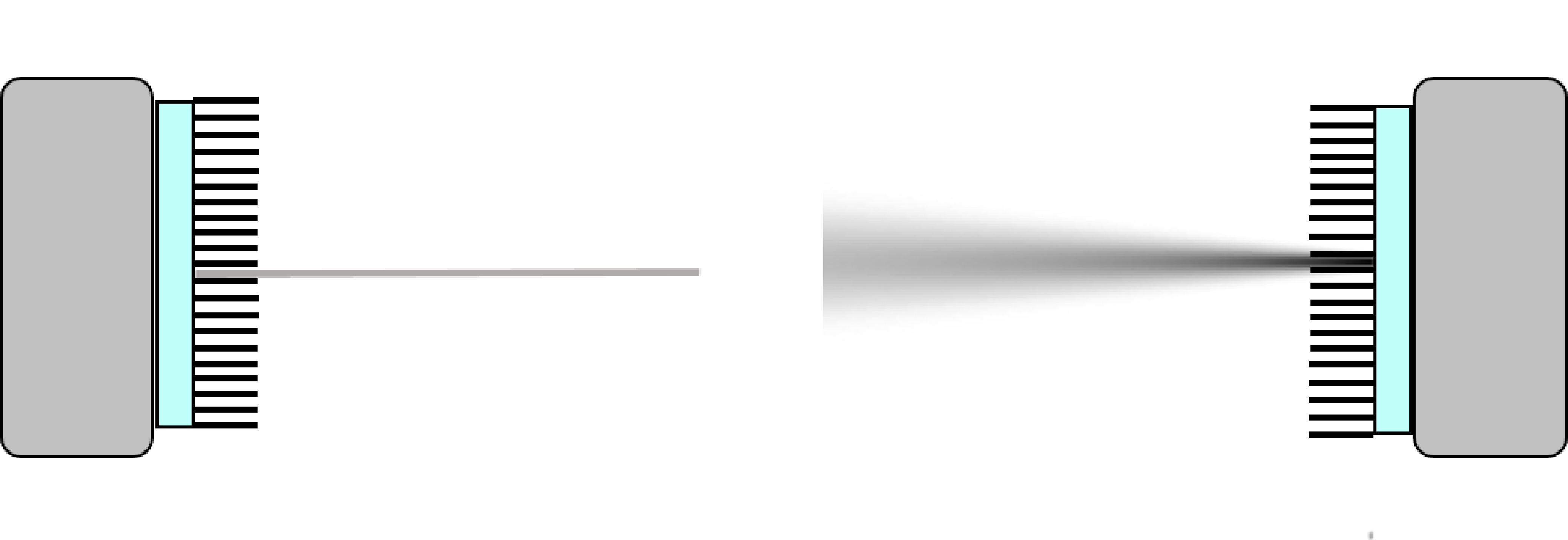
Figure 20:In a simple projector/backprojector, the projection is modeled as a (weighted) line integral. To account for the position dependent collimator blurring, the line integral can be replaced by a weighted integral over a cone.
In section Mechanical collimation in the gamma camera, we have seen that gamma cameras suffer from position dependent collimator blurring. As illustrated in Figure 20, this can be modeled by computing the projection not as a line integral, but as the integral over a cone, using appropriate weights to model the position dependent PSF. This position dependent blurring is then combined with the attenuation to obtain the system matrix elements . The same can be done for PET: the blurring due to the detector width (and if desired, also the positron range and/or the acolinearity) can be incorporated in the PET or TOF-PET system matrix elements.
During the iterations, MLEM (or OSEM) uses the system matrix in every projection and backprojection, and by doing so, it will attempt to invert all effects modeled by that system matrix. If the system matrix models a blurring effect, then MLEM will automatically attempt to undo that blurring. This produces images with improved resolution as illustrated for a SPECT and a PET case in Figure 21. Interestingly, modeling the finite system resolution in MLEM not only improves the resolution in the reconstructed image, it also suppresses the noise, as can be seen in the PET reconstruction.
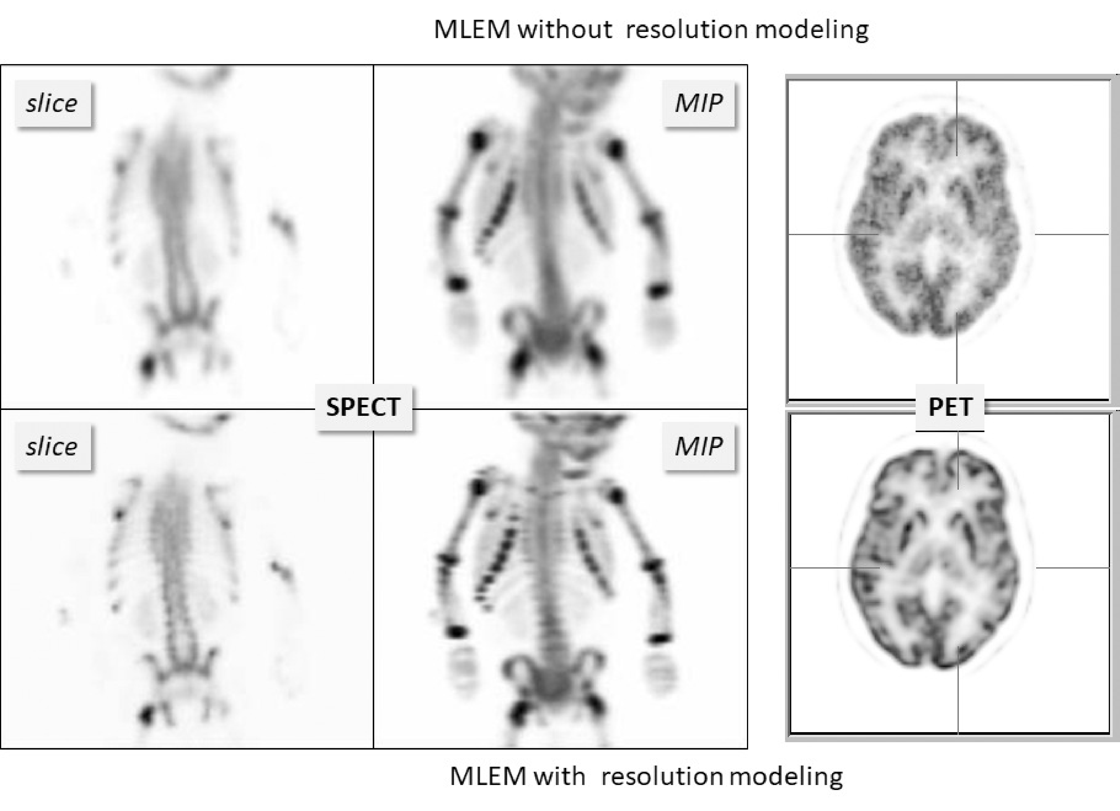
Figure 21:Reconstructions with and without resolution modeling from a SPECT bone scan of a child and a brain PET scan. “MIP” denotes “maximum intensity projection”. MLEM with resolution modeling recovers image detail that was suppressed by the finite system resolution.
However, the deblurring cannot be 100% successful, because deblurring is a very ill-posed problem. Except in special cases, deblurring problems have multiple solutions, and iterative algorithms cannot “know” which of those possible solutions they should produce. This is illustrated in Figure 22. A noise-free PET simulation was done, accounting for finite spatial resolution. MLEM images without and with resolution modeling were reconstructed from the noise-free sinogram. The figure shows that MLEM with resolution modeling produced a sharper image, but that image is different from the true image that was used in the simulation.

Figure 22:PET simulation without noise but with finite resolution modeling. MLEM with deblurring produced sharper images, but they are clearly different from the ground truth.
The problem is that the blurring during the projection not only suppresses some information, it also erases some information. MLEM can recover image details that have been suppressed but are still present in the data, but no algorithm can recover details that have been erased from the data. This can be best explained in the frequency domain.
Figure 23 shows a simple 1D thought experiment. In this experiment, we consider the PSF and its frequency spectrum. The frequency spectrum of the PSF is often called the modulation transfer function (MTF), because it tells us how the PSF of a system affects (modulates) all frequency components of a signal which is transferred through that system. Assume we are doing measurements on something that can be well represented by a 1D profile. The true profile has a single non-zero element. A measurement of that profile produces a blurred version of the true profile. We assume that the measurement device has a Gaussian PSF. The Fourier transform of a Gaussian is a Gaussian, so the Gaussian PSF corresponds to a Gaussian MTF; denoting the Fourier transform with , we have:
The wider the Gaussian PSF, the narrower the corresponding Gaussian MTF, and the larger the fraction of frequencies that are suppressed so much that they will be lost in the noise.
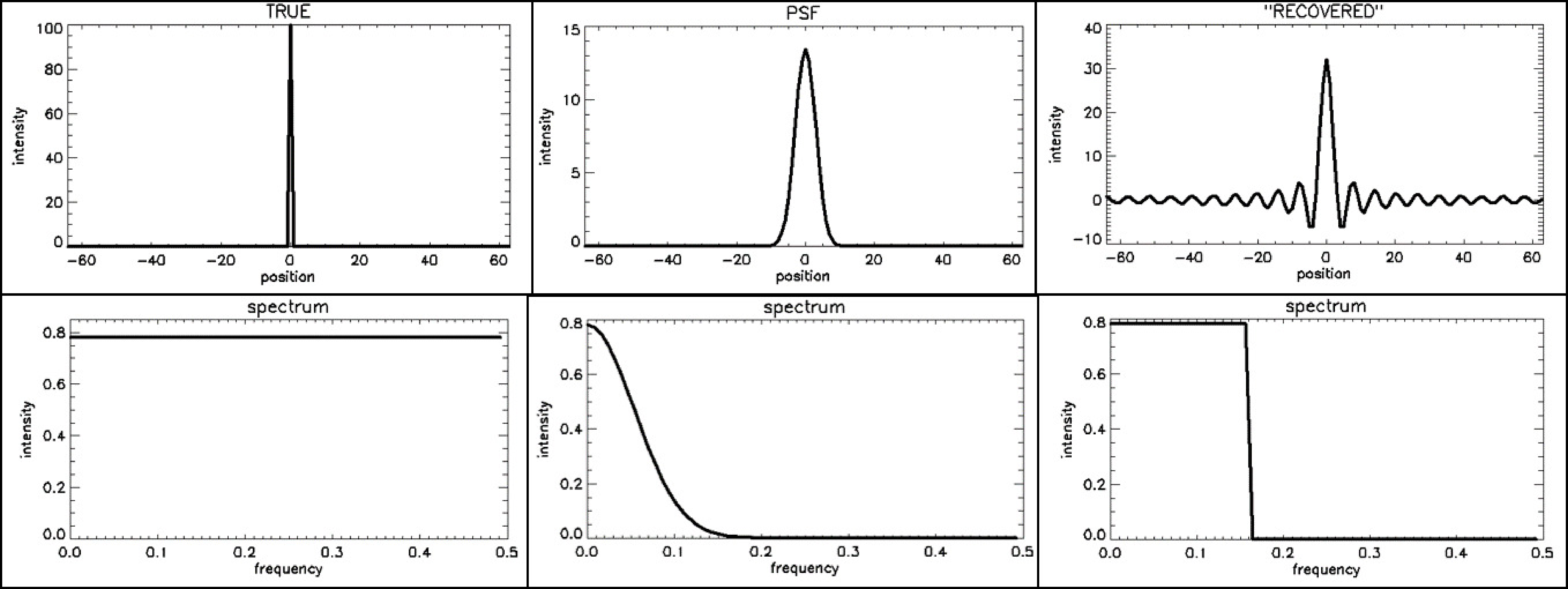
Figure 23:Impulse responses (top) and their corresponding frequency spectra or MTF (bottom). From left to right: (1) the ideal PSF (a flat MTF), a Gaussian PSF (Gaussian MTF) and a sinc-shaped PSF, corresponding to a rectangular MTF
Now imagine that we apply some deblurring algorithm, which restores the frequency components that are still present in the data. We also assume that it does not “invent” data, but assumes that things not seen by the measurement should be set to zero. That will result in an approximately rectangular PSF. This is illustrated in Figure 23, where we assumed that all frequencies below 0.16 could still be restored, whereas the higher frequencies were filtered away by the measurement PSF. The inverse Fourier transform of a rectangular function is a sinc function (), as can easily be verified:
where we used , and . Figure 23 shows a sinc function (to plot the function, make us of ). The PSF will oscillate at the cutoff frequency, so the wider the rectangular MTF, the narrower the central peak of the PSF and the narrower the ripples surrounding it.
Knowing the PSF, we can compute what the deblurred measurement will look like for any other signal, by convolving that signal with the PSF. Figure 24 shows the result for a block-shaped signal. The result is still block-like, but the two edges are less steep and are accompanied by ripples creating under- and overshoots. These ripples are often called Gibbs artefacts.

Figure 24:The convolution of a block-shaped signal with a sinc-shaped PSF produces a smoother version of the block with ripples, also called Gibbs artefacts, on top of it.
MLEM with resolution modeling combines reconstruction with deblurring for the system PSF, which is more complicated than simple deblurring. Nevertheless, when the system PSF is modeled during MLEM, very similar Gibbs artefacts are created, because MLEM cannot restore the higher frequencies that were lost due to that PSF. Because now the blurring and deblurring are done in three dimensions, the Gibbs artefact are rippling in 3D too. The effects in different dimensions can accumulate, and as a result, the over- and undershoots can become very large. E.g. for small hot objects, the overshoot can go as high as 100%. That is unfortunate, such high overshoots can cause problems for quantitative analysis of the tracer uptake in small hot lesions, as is often done in PET for oncology. Therefore, depending on the imaging task, it may be necessary to smooth the image a bit to avoid quantification errors due to these Gibbs effects.
The adjoint of a matrix is its conjugate transpose. Because the projection coefficients are real values, the adjoint of the projection matrix is its transpose.